How To Filter Excel Rows By Multiple Customized Condition

Microsoft Excel provides a filter function for you to find out required rows by the customized condition in a very long excel worksheet. The filter feature includes a basic filter that provides simple condition filtering and an advanced filter that provides complex condition filtering. This article will show you both the 2 filter features with examples.

1. Excel Basic Filter Example.

There is an example excel file which contains so many rows and each row contains a lot of columns, I want to focus on 2 columns, one is Country ( column B ) the other is Units Sold ( column E ). You can download the example file by click this link.

1.1 Filter Text Column (Country).

1. The Country column( column B ) is a text column, it contains some country text values like Canada, France, Germany, etc. I want to filter out the rows which Country column value is Canada or Germany. So I click the Excel Data —> Filter menu item in the top ribbon area. Then you can find there add a dropdown arrow at each column right side of the top header row.
2. When you click the Country column dropdown arrow to expand it, you can find some menu items such as Sort A to Z, Sort Z to A, Text Filters, etc. There is also a checkbox list at the bottom of the dropdown list, it summarizes all the country values that exist in the Country column such as Canada, France, Germany, etc.
3. If you click Sort A to Z or Sort Z to A list item, it will group the excel rows by the Country column value. If you only want to display the rows which Country column value is Canada or Germany, you can just check the checkbox before Canada and Germany checkbox and uncheck all other checkboxes. Then you will get all the excel rows that the Country column value is Canada or Germany.
4. If you think the filter condition is not enough for your scenario, you can click the Text Filters list item in the above header column drop-down list panel, and then add more complex text filter conditions through the popup menu list such as Does Not Equal, Begins With, Ends With, Contains, etc.
   
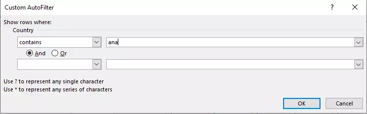
5. When you click one filter condition item for example Contains, it will popup a Custom AutoFilter dialog, you can input your filter condition in it.
   
6. You can add multiple filter conditions in the Custom AutoFilter dialog, for each condition, you can choose the operator from the first dropdown list, then input/select the values from the second dropdown list. You can also choose the relationship between the multiple conditions by selecting the And / Or radio button.
   

1.2 Filter Number Column ( Units Sold ).

1. Now we will add a simple filter to the Units Sold column ( column E ). Because this column contains number value, so there are some differences between it and the Country column which is a text column.
2. Click the dropdown arrow on the right side of the Units Sold column, you will see some list items. You can see the list item Sort Smallest to Largest, Sort Largest to Smallest, Number Filters, etc.
   
3. When you click the Number Filters list item, it will popup the number value filter condition menu list. Click one item such as Greater Than, and in the popup Custom AutoFilter dialog input 3000 after is greater than condition input box.
4. When you click the OK button in the above dialog, you can get all the excel rows that the Country column value is Canada or Germany and the Units Sold column value is greater than 3000.

2. Excel Advanced Filter Example.

In section 1, we had filtered out excel rows whose Country column value is Canada or Germany and Units Sold column value is greater than 3000. But how to filter out excel rows that match follow condition.

1. Country column value is Canada and Units Sold column value is greater than 3000.
2. Country column value is Germany and Units Sold column value is less than 500.

To filter out excel rows that match the above condition, we can use excel Data —> Advanced filter feature follow below steps.

1. Select the first excel worksheet row.
2. Click Home —> Insert —> Insert Sheet Rows to insert 5 rows at the worksheet top area.
3. Copy the original header row data ( now row 6 ) to the worksheet first row.
4. Add one filter condition in row 2, the condition is Country column value is Canada, and Units Sold column value is >3000.
5. Add another filter condition in row 3, the condition is Country column value is Germany, and Units Sold column value is <500.
6. I have created another worksheet Sheet2 in the example excel file for this example, and you can download it to see the effect.
7. After creating an advanced filter condition, we should click Data —> Sort & Filter —> Advanced menu icon to execute it, then it will pop up the Advanced Filter dialog.
8. Select the Filter the list, in-place radio button in the Advanced Filter dialog Action section.
9. In the Advanced Filter dialog, click the up arrow(↑) button at the end of the List range input text box, and input the filter query executed list range Sheet2!$A$5:$P$705 ( sheet_name!start_cell:end_cell ) in the input text box.
10. Click the up arrow(↑) button at the end of the Criteria range input text box, and input the filter condition list range Sheet2!$A$1:$P$3 ( sheet_name!start_cell:end_cell ) in it.
11. Click the OK button, now you can see the filtered out excel rows listed in the excel worksheet.
12. To clear the filter condition you should click Data —> Sort & Filter —> Clear item, then all the worksheet rows will be listed out.