How To Make A Table In Excel

The table is very useful in excel worksheets. Using a table can make your data more regular and manageable. You can sort data, filter data, etc. This article will show you how to make a table in excel cells and how to make it beautiful.

1. How To Make A Table In Excel Cells.

1. Create a worksheet and input the below data into it. The example data is car sales reports for different car brands in the months of January, February, and March.
   
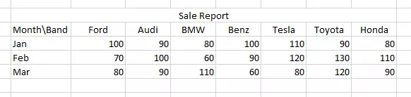
2. The title Sale Report cell has merged all it’s sibling cells. To do this, you should select all of it’s sibling cells and then click Home —> Merge & Center item in the Alignment group.
3. Now to create a table based on these cells, you should select all the data cells ( not include the title cell ( Sale Report cell ) ), then click Insert —> Table ( in Tables group ).
4. It will popup Create Table dialog. You should confirm the data cell range, if your table has headers you should check the My table has headers checkbox.
5. Click the OK button, it will translate the excel cell to the below table.
   
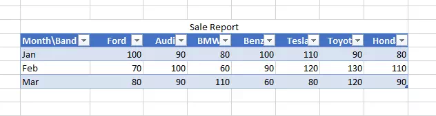
6. If you find the table header’s text is only partially visible, you can select the table and click Home —> Format ( in Cells group ) —> AutoFit Column Width menu item to expand header columns.

2. How To Add Table Border In Excel.

1. To add a border to the table, you can select the table ( include the title ( Sale Report ) cell ), and right-click it, then click Format Cells… menu item.
2. In the Format Cells popup dialog, click the Border tab, and then you can choose border line style, line color, and presets. Please note if you change the border style and color, you should reselect border Presets again to make the new border style and color take effect.
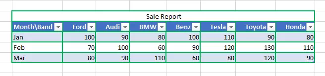
3. The below picture is the table that applied green border settings.
   

3. How To Sort / Filter Table Data Use Table Headers.

1. Each of the table headers has a dropdown arrow on the right side of the header, you can click it to sort table row data or filter out special table row data.
2. When you click the dropdown arrow, you can see menu items such as Sort Smallest to Largest, Sort Largest to Smallest, and the column values list with a checkbox before it. You can click each menu item or uncheck the checkbox to see the table row changes.

4. How To Apply Different Table Styles.

1. Excel provides a lot of built-in table styles for you to use. You can select the table style that you like follow the below steps.
2. Select any cell in the table.
3. Then you can see a Table Tools tab shown in the excel top ribbon area.
4. Click the Table Design tab, and you can select the table style in the Table Styles group.
5. Each built-in excel table style defines a different table border size, and color group.